Behaviour = Slope x Stimulus + residual
Although linear regression like this can be very powerful, and is often used to determine if two variables are linked (via correlation analysis), in general we cannot expect that animal behaviour is always so straightforwardly related to the stimuli or environmental cues we are interested in.
Consider for example how good you might feel over the course of an evening of heavy drinking. Here we can quantify the 'stimulus' as the number of drinks you consume. While some people are lucky enough to always consume in moderation to their acceptable intake, I would wager you have encountered evenings where your general state of enjoyment follows a trend like the one below.
 |
| Enjoy inference responsibly... |
How can we fit a function to a more complicated looking curve like this? One solution would be to try and guess the shape of the curve....but what function does it look like? If we choose badly then we'll never get a good fit to the data.
We'd like a more flexible alternative that doesn't require so much guesswork. To see how we can get there, first we need to understand how we might apply the previous straight line fitting techniques when we have multiple stimuli. Imagine we think that an animals behaviour is a function of two stimuli
Behaviour = f(Stimulus1, Stimulus2)
Well, how about starting by extending the equation we had for a straight line. The original equation for just one stimulus was:
Behaviour = Slope x Stimulus + residual
For reasons that will become clear, we can draw this relationship using the following schematic

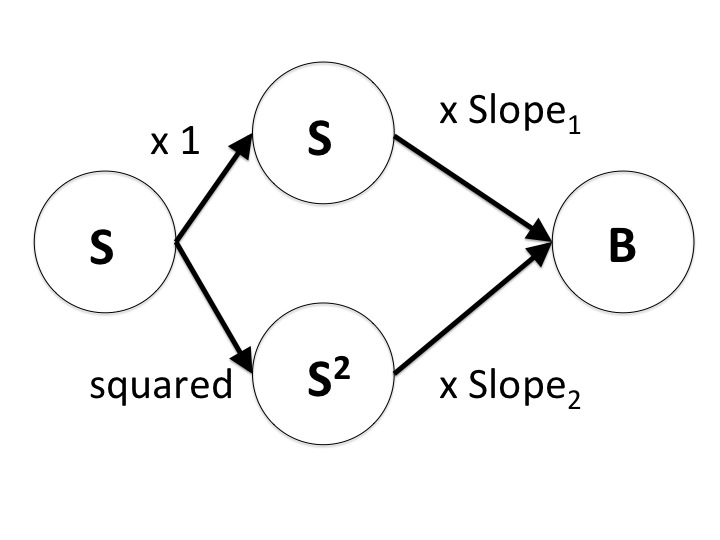
Extending this to two stimuli we have two slopes:
Behaviour = Slope1 x Stimulus1 + Slope2 x Stimulus2 + residual
and similarly a new picture, showing that the behaviour comes from adding the two different factors:

Now the behaviour varies in response to both stimuli. Each slope tells us how strong the relationship between stimulus and behaviour is, and we can find out what these slopes are in much the same way as before, either by trying different values until we get the lowest squared-sum-of-errors (see the last post), or by using the special formulae that exist for telling us the best solution. I don't intend to worry about these formulae here, but if you want to find them or see where they come from then the Wikipedia page on Ordinary Least Squares is a good place to look.
We can extend this basic approach further, including more and more stimuli. But, at this point you may be wondering "How does this help us fit functions like the one about drinking enjoyment above?" At this point we employ a wonderful little trick. Remember we talked about guessing the form of that function? I said that this would be too restrictive. But what if we guess lots of functions?
The trick here can be seen simply by taking the equation for two stimuli we had above, but now imagine that stimulus 2 is related to stimulus 1. Instead of two different stimuli, imagine instead that we replace stimulus 2 with a function of stimulus 1. Lets try something simple, like Stimulus12.
Behaviour = Slope1 x Stimulus1 + Slope2 x Stimulus12 + residual
Now, if we find the best fit values for these slopes, based on the observed values of Stimulus1 and Stimulus12 we are actually fitting a non-linear, quadratic function to the data. If we know what Stimulus1is then we can easily calculate Stimulus1^2, and then we can treat them as if they were different stimuli. Fitting this function is still the same process as before - we choose different values for the slopes and find those that produce the lowest residual errors. See that our schematic of the model now has an additional layer between the stimulus and the behaviour.
We can take this simple trick further. Instead of many stimuli, we can use many different functions of the same stimulus. Consider a set of different functions of the stimulus, gi(stimulus), where each value of i specifies a different function. We can model the behaviour as being a sum of these functions, each with its own slope
Behaviour = Slope1 x g1 (Stimulus) + Slope2 x g2 (Stimulus) + Slope3 x g3 (Stimulus)... etc
These functions could each be different powers of Stimulus, giving us a polynomial fit, or they could be any other set of functions. The key point here is that instead of guessing one kind of function to fit, we can try lots of different functions and weight them according to how important they are. Just as in every case before, when we try different values for the slopes, we get different residual errors, and we aim to find the best values that minimise those errors. Of course, as the number of slopes increases it becomes harder to find the best values easily, but in principle the task is the same.
The schematic of this kind of model (below) shows that we now have an expanding middle layer, where each circle represents a different function of the stimulus. The value of Stimulus is passed to each of these functions. The output of each function is then weighted according to the value of its Slope and passed to the Behaviour, which is made from the sum of all these bits.

The next and final stage is to consider developing this middle layer one step further, so we can once again consider multiple different stimuli. Instead of just one stimulus at the start which leads to our middle layer, imagine we have many stimuli to consider. Each function in the middle layer is now dependent on all the different stimuli, so e.g. g1 = g1 (S1 , S2 , S3 ...). Connect each stimulus to every function in the middle layer...
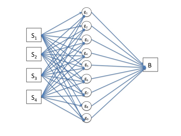 |
| Don't worry about the switch from circles to squares or from black arrows to blue, I'm just reusing an old image! |
Now we have a model which is going to look very complicated if we write it down as an equation. In essence though the idea remains the same as our first linear model. Along each line we simply multiply the input by some number, just like the slope of the linear plot. The behaviour predicted by the model is given by adding up all the different bits coming out of the middle layer into the final node, and we can adjust the multiplying numbers on each line to get the lowest error possible. When we find the best values for these numbers we have something which acts as a function taking stimuli to behaviour. We can then put it any value of stimuli we are interested in and see what the function predicts the animal will do.
You may have seen something like the above picture before. It is an example of what is known as an artificial neural network and is of a special type called a multi-layer perceptron. In such models the functions in the middle layer are usually sigmoidal functions that aim to mimic the highly thresholded response of real neurons to stimuli in the brain. Each function takes in a weighted sum of the stimuli, S, and sends out an output according to a profile like that below.
You may have seen something like the above picture before. It is an example of what is known as an artificial neural network and is of a special type called a multi-layer perceptron. In such models the functions in the middle layer are usually sigmoidal functions that aim to mimic the highly thresholded response of real neurons to stimuli in the brain. Each function takes in a weighted sum of the stimuli, S, and sends out an output according to a profile like that below.
 |
These neural networks provide us with a tool which can fit extremely variable non-linear functions of many stimuli. Neural networks have a lot of parameters that can be varied, each one essentially like the slopes we learnt for the linear model. Just as before, when these parameters are changed they alter the residual error between the behaviour predicted by the model and the observed behaviour. Unfortunately there is no general solution that quickly tells us what these parameters should be like there was for the linear model, but there are lots of clever ways to find good values for these parameters by iteratively changing them, making sure the error keeps going down. But this is a long way beyond the scope of today's post.
Obviously a short blog post like this leaves many aspects of this kind of model fitting unaddressed, such as how we learn the parameters, or which functions we use for the middle layers. Although I have tried to give you some idea how such a model works by relating it back to the linear straight line fitting, the important thing to remember is what we shall see in the next post: you can use models like this while understanding almost nothing of what is going on inside. Lots of computer scientists have generously studied these sorts of models for decades, creating neat little toolboxes like Netlab for Matlab that allow us to fit complicated functions without getting our hands dirty with the modelling machinery! The important thing is to be secure enough in knowing what is going on in principle that you are happy to look away and let the toolbox do its work. In the next post I will try and show, with a bit of Matlab code, how we actually apply a neural network from this toolbox to (finally!) learn how fish shoal...
[If you are interested in more of the details surrounding this topic, I can highly recommend David Mackay's textbook, Information Theory, Inference and Learning Algorithms (free online) - try Section V]
Hey there,
ReplyDeleteI am really happy to say it’s an interesting post to read. I learn new information from your article, you are doing a great job. Keep it up visit Gift card generator 2019